
The cut-off is a popular word during the admission season, especially in India. For us at Questionbang, the cut-off is something often asked by mock-set-plus users – Has my score is good enough to qualify Joint Entrance Examination (JEE)? Hence, we decided to predict the cut-off for the next season and have it in result analysis.
Background
Most of us have used basic regression analysis during our class 12th maths, e.g, time series and forecasting. In reality, the outcomes of such predictions are going to be dependent on various factors. The use of simple regression may not be sufficient in such cases.
Let us consider our requirement – predicting cut-off marks for JEE. The table below shows cut-off scores for the last 6 years.
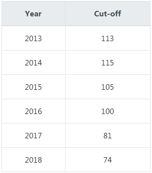
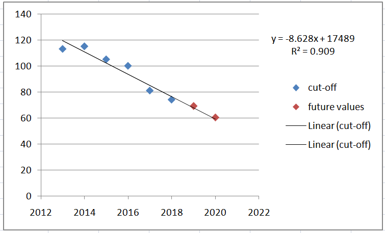
Let us try a simple curve fitting approach (Figure 1); this is giving a prediction of 69 for the year 2019. However, we cannot relate these points to any reasoning. As we can see, the cut-off (Y) was 113 for the year 2013 and became 74 in 2018 (Table 1). Surely many factors influence the cut-off.
PRACTICE JEE ONLINE TESTS >>
Assumptions
Let us assume those cut-offs (Table 1) are a measure of competition and hence, are a function of the following variables:
- Number of seats available (
 ),
), - Difficulty level (),
- Number of applicants ().
How these individual variables influence the outcome is something to be predicted.
Choosing a regression method
What is the regression analysis?
In statistical modeling, regression analysis is a set of statistical processes for estimating the relationships among variables. It includes many techniques for modeling and analyzing several variables when the focus is on the relationship between a dependent variable and one or more independent variables [wiki].
There are many different types of regression techniques. They are mainly of two categories – linear regression and non-linear regression.
In our case, the cut-off score (predictor) is dependent on three independent variables ( ,
,  ,
,  ) as discussed before. Hence, this is going to be a multiple linear regression scenario.
The table below (Table 2) is an extension of Table 1 (Cut-off scores for the last 6 years) to include the number of seats available, difficulty level and the number of applicants.
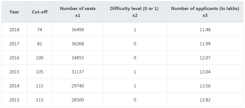
The difficulty level is a categorical variable having level 1 (high) or 0 (moderate).
About data
The data – cut-off scores, seat availability, number of applicants and difficulty level have been gathered from online news portals. The JEE format changed a few times during the past 20+ years. It has a two-phase (Mains & Advanced) format since 2013. We will use data from 2013 to 2018.
PRACTICE JEE MOCK TESTS >>
Revisiting the basics of least square regression method – a single independent variable condition
Assume a single independent variable condition and set of values as below (Table 3). Let us call these observations.
 |
 |
 |
|
 |
|
 |
|
 |
 |
Table 3. Observations.
– Independent variable,
– Actual dependent variable.
Following is an equation for simple linear regression:
(1)

Let us compute predictions  , using the the above values (Table 3):


 .
.
In generic form, the equation for predicted value will become:
(2)

|
|
 |
|
|
 |
|
|
 |
|
|
|
|
|
 |
Table 4. Observations and predictions.
– Predicted value.
Let us verify the accuracy of our prediction (Table 5),
|
|
|
 |
|
|
|
 |
|
|
|
 |
|
|
|
|
|
|
|
 |
Table 5. Observations, predictions and errors.
= error term.
As you can see, we subtracted the predictions () from the actual observations () to compute errors (). The next objective would be to refit the line so that the error () is minimized.
(3)

From (2) and (3),
(4)

Eq (4) is a squared error function; we need to find coefficients a & b to achieve minimum (zero) error. Take the partial derivative of eq (4) with respect to a and b:
(5)

(6)

From (5) and (6),
 (7)
 (8)


PRACTICE FREE JEE MOCK TESTS ONLINE >>
Computing JEE Cut-off – three independent variable condition
In our case, we have three independent variables – , , and coefficients –  ,
,  ,
,  ,
,  . The regression equation becomes,
(9)

Intercept a is:
 (10)
(10)where;
 ,
,  and
and  are means of respective variable values.
And the normal equations are,
(11) 
(12) 
(13) 
Writing the above equations in matrix form and solving using Cramer’s rule:
![b=\frac{\sum{y_ix_1}[\sum{x_2^2}\sum{x_3^2}-(\sum{x_2x_3})]-\sum{x_1x_2}[\sum{yx_2}\sum{x_3^2}-\sum{yx_3} \sum{x_2x_3} )] + \sum{x_1x_3}[\sum{yx_2}\sum{x_2x_3}-\sum{yx_3} \sum{x_2}^2 )] }{\sum{x_1^2}[\sum{x_2^2}\sum{x_3^2}-(\sum{x_2x_3}^2)]-\sum{x_1x_2}[\sum{x_1x_2}\sum{x_3^2}-\sum{x_1x_3} \sum{x_2x_3} )] + \sum{x_1x_3}[\sum{x_1x_2}\sum{x_2x_3}-\sum{x_1x_3} \sum{x_2}^2 )]}, (14)](https://www.questionbang.com/blog/wp-content/ql-cache/quicklatex.com-e3fe4529e3de5110b03bce53f6142264_l3.png "Rendered by QuickLaTeX.com")
![c=\frac{\sum{x_1^2}[\sum{yx_2}\sum{x_3^2}-(\sum{yx_3})]-\sum{yx_1}[\sum{x_1x_2}\sum{x_3^2}-\sum{x_1x_3} \sum{x_2x_3} )] + \sum{x_1x_3}[\sum{x_1x_2}\sum{yx_3}-\sum{x_1x_3} \sum{yx_2})] }{\sum{x_1^2}[\sum{x_2^2}\sum{x_3^2}-(\sum{x_2x_3}^2)]-\sum{x_1x_2}[\sum{x_1x_2}\sum{x_3^2}-\sum{x_1x_3} \sum{x_2x_3} )] + \sum{x_1x_3}[\sum{x_1x_2}\sum{x_2x_3}-\sum{x_1x_3} \sum{x_2}^2 )]}, (15)](https://www.questionbang.com/blog/wp-content/ql-cache/quicklatex.com-1c4698234decbcf72b27b4717a2c10cd_l3.png "Rendered by QuickLaTeX.com")
![d=\frac{\sum{x_1^2}[\sum{x_2^2}\sum{yx_3}-\sum{x_2x_3} \sum{yx_2}]-\sum{x_1x_2}[\sum{x_1x_2}\sum{yx_3}-\sum{x_1x_3} \sum{yx_2} )] + \sum{yx_1}[\sum{x_1x_2}\sum{x_2x_3}-\sum{x_1x_3} \sum{x_2^2})] }{\sum{x_1^2}[\sum{x_2^2}\sum{x_3^2}-(\sum{x_2x_3}^2)]-\sum{x_1x_2}[\sum{x_1x_2}\sum{x_3^2}-\sum{x_1x_3} \sum{x_2x_3} )] + \sum{x_1x_3}[\sum{x_1x_2}\sum{x_2x_3}-\sum{x_1x_3} \sum{x_2}^2 )]}. (16)](https://www.questionbang.com/blog/wp-content/ql-cache/quicklatex.com-3dc351f71772f47994dee1a70691ac6c_l3.png "Rendered by QuickLaTeX.com")
PRACTICE FREE JEE TEST SERIES >>
Let us calculate the coefficients a, b, c and d using Microsoft Excel.
(Courtesy: https://onlinecourses.science.psu.edu/stat501/node/380/)
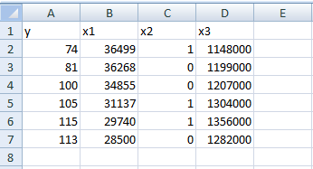
Using data analysis toolkit in MS Excel:
a = 26.0402,
b = -0.00225,
c = -6.4645,
d = 0.000119.
After substituting the above coefficients, eq (9) becomes,
(17)

We can use the above eq (17) to compute the JEE cut-off.
We will assume the following values for the year 2019:
Number of seats () = 36500,
Difficulty level () = 1 or 0,
Number of applicants () = 11 lakh.
A) Using eq (10), high difficulty ( )
)
 |
 . . |
B) Using eq (10), moderate difficulty ( )
)
 |
 . . |
Cut-off score range:  – –  . . |
Conclusion
The above prediction may not be accurate as it is based on a very limited set of data. It is to be noted that, this prediction is not relevant for the year 2019 (onwards), as the cut-off is going to be in percentile not in the score.
Questionbang users can find these values in the mock-set-plus result analysis section.
We value your feedback and welcome any comments to help us serve you better.
References:
- https://www.questionbang.com/site/result-analysis
- https://www.questionbang.com/site/mock-set-plus/jee
- https://www.questionbang.com/
- https://www.questionbang.com/ws/
- https://onlinecourses.science.psu.edu/stat501/node/380/
- https://en.wikipedia.org/wiki/Cramer%27s_rule
- https://en.wikipedia.org/wiki/Regression_analysis
- https://en.wikipedia.org/wiki/Microsoft_Excel